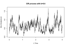
In mathematical finance, the Cox–Ingersoll–Ross (CIR) model describes the evolution of interest rates. It is a type of "one factor model" (short-rate model) as it describes interest rate movements as driven by only one source of market risk. The model can be used in the valuation of interest rate derivatives. It was introduced in 1985[1] by John C. Cox, Jonathan E. Ingersoll and Stephen A. Ross as an extension of the Vasicek model, itself an Ornstein–Uhlenbeck_process.

The model

The CIR model describes the instantaneous interest rate 
where 


The standard deviation factor, 


is met. More generally, when the rate (

In the case 
Distribution
- Future distribution
- The distribution of future values of a CIR process can be computed in closed form:
- where
, and Y is a non-central chi-squared distribution with
degrees of freedom and non-centrality parameter
. Formally the probability density function is:
- where
,
,
, and
is a modified Bessel function of the first kind of order
.
- Asymptotic distribution
- Due to mean reversion, as time becomes large, the distribution of
will approach a gamma distribution with the probability density of:
- where
and
.
Derivation of asymptotic distribution |
|---|
To derive the asymptotic distribution Our interest is in the particular case when Defining Integrating shows us that: Over the range |
Properties
- Mean reversion,
- Level dependent volatility (
),
- For given positive
the process will never touch zero, if
; otherwise it can occasionally touch the zero point,
, so long term mean is
,
Calibration
- The continuous SDE can be discretized as follows
- which is equivalent to
- provided
is n.i.i.d. (0,1). This equation can be used for a linear regression.
- Martingale estimation
- Maximum likelihood
Simulation
Stochastic simulation of the CIR process can be achieved using two variants:
- Discretization
- Exact
Bond pricing
Under the no-arbitrage assumption, a bond may be priced using this interest rate process. The bond price is exponential affine in the interest rate:
where
Extensions
The CIR model uses a special case of a basic affine jump diffusion, which still permits a closed-form expression for bond prices. Time varying functions replacing coefficients can be introduced in the model in order to make it consistent with a pre-assigned term structure of interest rates and possibly volatilities. The most general approach is in Maghsoodi (1996).[2] A more tractable approach is in Brigo and Mercurio (2001b)[3] where an external time-dependent shift is added to the model for consistency with an input term structure of rates.
A significant extension of the CIR model to the case of stochastic mean and stochastic volatility is given by Lin Chen (1996) and is known as Chen model. A more recent extension for handling cluster volatility, negative interest rates and different distributions is the so-called "CIR #" by Orlando, Mininni and Bufalo (2018,[4] 2019,[5][6] 2020,[7] 2021,[8] 2023[9]) and a simpler extension focussing on negative interest rates was proposed by Di Francesco and Kamm (2021,[10] 2022[11]), which are referred to as the CIR- and CIR-- models.
See also
References
Further References
- Hull, John C. (2003). Options, Futures and Other Derivatives. Upper Saddle River, NJ: Prentice Hall. ISBN 0-13-009056-5.
- Cox, J.C., J.E. Ingersoll and S.A. Ross (1985). "A Theory of the Term Structure of Interest Rates". Econometrica. 53 (2): 385–407. doi:10.2307/1911242. JSTOR 1911242.
{{cite journal}}: CS1 maint: multiple names: authors list (link) - Maghsoodi, Y. (1996). "Solution of the extended CIR Term Structure and Bond Option Valuation". Mathematical Finance. 6 (6): 89–109. doi:10.1111/j.1467-9965.1996.tb00113.x.
- Damiano Brigo; Fabio Mercurio (2001). Interest Rate Models — Theory and Practice with Smile, Inflation and Credit (2nd ed. 2006 ed.). Springer Verlag. ISBN 978-3-540-22149-4.
- Brigo, Damiano; Fabio Mercurio (2001b). "A deterministic-shift extension of analytically tractable and time-homogeneous short rate models". Finance & Stochastics. 5 (3): 369–388. doi:10.1007/PL00013541. S2CID 35316609.
- Open Source library implementing the CIR process in python
- Orlando, Giuseppe; Mininni, Rosa Maria; Bufalo, Michele (2020). "Forecasting interest rates through Vasicek and CIR models: A partitioning approach". Journal of Forecasting. 39 (4): 569–579. arXiv:1901.02246. doi:10.1002/for.2642. ISSN 1099-131X. S2CID 126507446.


