User:Peter Mercator/Draft for Mercator

Mercator's map was described as a planisphere^[1] measuring 202 cm by 124 cm, printed on eighteen separate sheets. It is entitled Nova et aucta orbis terrae descriptio ad usum navigantium emendate accommadata, that is “A new and enlarged description of the Earth with corrections for use in navigation”. The map shown below is available in much higher resolution at Mercator 1569 world map where, in addition, may be found the Latin map legends with English translations as well as descriptions of some of the important features such as the Organum Directorium (lower right) and the two magnetic poles.

In the map legend centred on North America, titled "Greetings to the reader", Mercator gives an explanation of his aims.

"In this mapping of the world we have [desired] to spread out the surface of the globe into a plane that the places should everywhere be properly located, not only with respect to their true direction and distance from one another, but also in accordance with their true longitude and latitude; and further, that the shape of the lands, as they appear on the globe, shall be preserved as far as possible. For this there was needed a new arrangement and placing of the meridians, so that they shall become parallels, for the maps produced hereto by geographers are, on account of the curving and bending of the meridians, unsuitable for navigation. Taking all this into consideration, we have somewhat increased the degrees of latitude toward each pole, in proportion to the increase of the parallels beyond the ratio they really have to the equator."

The map title and this detailed statement clearly show that Mercator devised his map with navigators in mind and it must be considered as primarily a chart for mariners -- although he was unable to resist the temptation to add highly speculative geographical detail to the interior of the non-European continents. Mercator did not achieve all of his desiderata. Whilst the map preserves angles it does not preserve distances: it is impossible to do both.

In the sixteenth century mariners used plane charts based on a portion of the equirectangular projection (or plate carrée projection) of the globe. This is the simplest and most venerable projection, its first known use, around 100AD, was by Marinus of Tyre^[2] to whom Ptolemy^[3] had ascribed the invention. In its simplest form^[4] the meridians and parallels form a square grid, the important properties for this case are

• The scale is constant and correct on every meridian.
• The scale is constant and correct on the equator.
• The scale is neither constant nor correct on any other line. (Consider the right angled triangle with base on a parallel and upright on a vertical. These lengths can be correctly placed on the plane chart but the hypotenuse calculated with Pythagoras will be wrong).
• The poles, which are points on the globe, become lines across the full width of the projection
• The scale on a parallel increases from unity at the equator to infinity at the poles.
• Scale distortion is indicated on the figure by the ellipses. There is no stretching in the vertical direction but the horizontal distortion increases with latitude.

• A great circle route (black), defined by the intersections of the surface of the globe and planes through its centre, does not project to a straight line on the projection.
• A rhumb line (red) does not project to straight line on the projection.

The first and last properties are central to the discussion of the Mercator projection. Briefly, Mercator constructed a non-constant meridian scale such that rhumb lines do project to straight lines. Rhumb lines are the simplest possible sailing courses, a constant bearing such that the angle between the rhumb and every meridian it crosses is constant. In general, if such a path is extended at both ends it spirals to the poles, the total line being of finite length. The exceptions are rhumbs at a constant latitude which are closed parallel circles on the globe, equator included.

Early medieval charts had no indications of latitude or longitude but the location of known features confirms their dependence on the plane-chart equirectangular projection.By the middle of the sixteenth century this dependence is often made explicit by a latitude scale on the map. The example shown is a 1571 chart by the Portugese cartographer Fernão Vaz Dourado (c1520—c1580). The latitude is clearly a linear scale and the grid is square. The straight lines criss-crossing the chart are drawn from the points of the compass rose but the interpretation of these lines by mariners was at fault. Some claimed that they were rhumbs, some claimed they were great circles, some even claimed they were both, having mistakenly identified rhumbs as lines of shortest distance. The inadequacies of their charts for accurate sailing were well known, if not understood, and mariners coped by supplementing the charts with "rule of thumb" corrections preserved in their oral tradition. Their problems were also compounded by inadequate instruments for the determination of latitude and longitude (sextant, chronometer) and a lack of knowledge of magnetic deviation. Nevertheless, mariners persisted in using plane charts for a hundred years aftre the appearance of Mercator's chart.

The Portugese mathematician and cosmographer Pedro Nunes (1502—1578) was the first to clarify some of the issues concerning charts. He described the rhumb line (loxodrome) and its use in navigation and proved^[5] that it was spiral line extending to the poles. He also proved that the shortest distance between two points was an arc of a great circle of the sphere (the orthodrome), not the rhumb (loxodrome).

Nunes was also in contact with the Englishman John Dee(1527–1608)— mathematician, alchemist and a navigational adviser to the Muscovy Company. He also investigated the rhumb and calculated,^[6], the position of points on the globe which lay on the seven standard rhumbs of the sphere (at the compass points of 11¼, 22½, 33¾, 45, 56¼, 67½ and 78¾ degrees).

Mercator knew of the work of Nunes and, in 1541, he constructed^[7] a globe showing rhumb lines as distinct from great circles. He did not describe the method of construction but it is possible that he simply used a metallic template for each rhumb angle. From a point on the starting meridian he could draw a straight line to the 'next' meridian, then draw a second section and so on. This segmented line will approach a smooth curve as the step to the next meridian is decreased. There is no evidence that Mercator knew of Dee's calculations (although the two had met at an earlier date.^[8]).

Mercator's genius was to conceive that it was possible to derive a planisphere from a globe showing rhumb lines in such a way that the rhumb lines became straight lines. He left no details of his method, other than his statement about having "somewhat increased the degrees of latitude toward each pole", and there have been only speculative suggestions.^[9] The following construction starts from the assumption that one is in possession of a globe augmented with rhumb lines. First, measure the latitude-longitude values at a number of points on one or more rhumb lines drawn on the globe, and then plot these points on the plane chart and connect them by a smooth curve (red). In the figure (left) the points were measured on a rhumb line at 45° on the sphere passing through the point with zero latitude and longitude. (For simplicity only a quarter of the chart is shown—for northern latitudes from Greenwich to 180°E). The resulting rhumb line on the plane chart is not a straight line. Compare the rhumb with the straight line (green) which has the same slope as the rhumb at its starting point, 45°. The vertical blue lines then show the amount by which the parallels must be adjusted so that the rhumb is straightened; this construction gives the spacing for the Mercator parallels shown on the right. However Mercator proceeded, his method must have been logically equivalent to the above construction; any inaccuracies in constructing and measuring the rhumbs on the sphere, and in transferring positions to the chart, would give errors in the positions of he parallels.

Misconception I: The Mercator projection is a geometrical projection

There is a widespread misconception that the spacing of the parallels in Mercator's projection is described by a literal geometrical projection from the centre of a model globe, as if a light at the centre was projecting an outline of the surface features on to a cylinder tangential to the equator. This is WRONG: the spacing of Mercator's parallels is quite different. The geometrical projection from the centre defines the Central Cylindric projection^[10]. It stretches to infinity faster than Mercator and the distortion at high latitudes is much worse. The Central Cylindric projection has no practical uses other than as an illustration of a purely geometric projection.

Misconception II :Erhard Etzlaub constructed an earlier version of the projection

It has been conjectured that Mercator "may" have seen the miniature "compass maps" of the German instrument maker Erhard Etzlaub (c. 1460–1532): such maps were used to calibrate the sundials at different latitudes. In 1917, Joseph Drecker^[11] had examined the 1513 miniature map and declared it to be a Mercator projection. The map covers latitudes from the equator to 67° with parallels at spacings similar to those of Mercator's projection— the scale shown on the left of the map. There are no meridians shown but they can be identified from cartographic features. Wilhelm Krücken^[8] has made a careful analysis of both Etzlaub's und Mercator's maps and he concludes that the principles of construction are different and the Etzlaub maps should not be considered as progenitors of Mercator's projection. Krücken showed that the Mercator map scaled so that the equatorial widths are equal to those of Etzlaub would have have the latitude scale appended to the right side of the Etzlaub map—these are quite different.

Conformality is the property which distinguishes the Mercator projection from other cylindric projections: moreover, it is the only such cylindric projection. In the context of the Mercator projection conformality is essentially equivalent to the statement "rhumb lines go to straight lines", but there are two other precisely equivalent statements and one other approximate statement. The discussion here is qualitative: a mathematical discussion is given later in this article (below).

Equality of angles

Any line (blue in figure) through a point P on the sphere must be tangential to some rhumb line (red) through P; on the projection the angle between both lines and the meridian is unchanged. Therefore the angle between an arbitrary line and the meridian is conserved. At B the angle between two intersecting lines and the meridian is conserved so the angle between them is conserved, i.e. the angle between any two lines at their point of intersection is conserved, as at C. This local property of angle conservation at a point is normally taken as the definition of conformality in mathematical texts. One practical implication is that the projection accurately renders such features as the twists and turns of rivers or coastlines, for they may be approximated by many short line segments and the angle between successive segments is always correct.

Equality of scale factors

Consider a small segment of an arbitrary line on the sphere, small enough so that the parallels and meridians bounding it define an approximate rectangle, as shown in the previous figure at D. The corresponding segment on the projection is bounded by an exact rectangle. Conservation of angle means that the ratios of the sides and diagonals of the elements must be the same and therefore the scale factors along the parallel (P'M'/PM), along the meridian (P'K'/PK) and along the diagonal (P'Q'/PQ) must be equal. The common value of these equal scale factors by is denoted here by the symbol k. Since the element on the sphere is only a rectangle in the limit of vanishing size it is more correct to stress that the point scale factors in all directions at P are equal. This statement of equal scale factors is entirely equivalent to the statement of angle conservation and vice-versa: either may be taken as a definition of conformality.

On the Mercator projection all parallels are projected to the same length as the projected equator.For example, at a latitude of 30 degrees the length of a parallel circle is 0.866 times the length of the equator so the scale factor on the map parallel is 1/0.86=1.15. At 60 degrees the parallel circle has a length of one half that of the equator so the scale factor along that parallel on the map is 2. In this way one can construct the figure (right) which shows the scale factor as a function of latitude; Since the parallel circles shrink to zero length at the pole the scale factor tends to infinity as the pole is approached. The divergence of scale at the poles is a major weakness of the Mercator projection, rendering it unsuitable at high latitudes. On the other hand, at low latitudes the scale distortion is small so that the projection is well suited for accurate mapping in equatorial regions. (Accuracy is within 1% at 8 degrees and within 5% at 17 degrees).

Whilst the scale along a parallel is constant, the equality of the parallel and meridian factors at any point implies that the meridian scale factor changes continuously along the meridian. Only point scale is meaningful on the meridian. Similarly the point scale along any path other than a parallel changes with latitude. Such scale variation complicates distance measurements on the Mercator map. If there is a bar scale on the map it will be true only on the equator: nowhere else. One could have a series of bar scales giving the scale factors on other parallels (example here), but this doesn't solve the problem of measuring distances in other directions. Mercator's method, explained on his map, uses the Organum Directorium in the bottom right hand corner of the map. The distance problem is also discussed in the section on nautical charts and the in the mathematical section below.

Approximate shape preservation

Since the scale factor is independent of direction it follows that small area elements on the sphere are stretched equally in all directions so that shape is preserved. The qualifier 'small' means that the scale factors must not vary perceptibly over the extent of the feature under examination. However, since there must always be some variation of scale over any finite area, the property of shape preservation (the literal meaning of conformal) is an approximate property of the projection. The figure illustrates that small shapes are preserved but the large green element is magnified and distorted. A comparison of the Mercator projection with a model globe shows that small features are well shaped. Madagascar, near the equator, is very good but small islands at higher latitudes, like Iceland or Tasmania, are still fairly good. However, the variation of the scale factor over Greenland distorts its shape in addition to its size.

Area is not conserved

No conformal map can also conserve area. In the Mercator projection, area distortion, increasing by a factor which is the product of the parallel and meridian scale factors, rapidly becomes worse at high latitudes. At 60N the parallel and meridian scale factors are both equal to 2 and the area scale is 4. Greenland, at even higher latitudes, is shown as having roughly as much land area as Africa whereas the true areas are in the ratio 1/14.

Edward Wright (1561–1615)

The mathematical investigation of the Mercator projection was initiated by a Cambridge professor, Edward Wright (1561–1615), who moved to London in 1596 to become a navigational adviser to the East India Company. In his 1599 publication, entitled Certain errors in navigation^[12], he explains how the spacing of the parallels could be calculated accurately using a table of cumulative secants (or meridian parts): see below for mathematical details . He was of course criticising Mercator and, in the 1610 edition, his comments were made explicit: "by occasion by that mappe of Mercator, I first thought of correcting so many, and grosse errors, and absurdities, as I haue alreadie touched. How this should be done, I learned neither of Mercator nor of any man else".

Wright's method^[12] is very simple, requiring very little in the way of mathematics. Consider the relation between the sphere and the plane chart, where the scale along meridians is equal to that along the equator but each parallel is stretched by a scale factor equal to the length of the equator divided by the proper length of the parallel on the sphere. For example the parallel at 60°, has to be stretched a factor of 2 in going from sphere to chart. Divide the upper half of the plane chart into 9 strips divided by the parallels at 10°, 20° etc., and let the width of each strip of the plane-chart be w. Approximate equality of parallel and meridian scales will be maintained over this strip if both scale factors are approximated by the value of the parallel scale factor at mid-latitude. For example the strip from 50° to 60° is stretched by the scale factor along the parallel at 55°: since this is 1.7 the width is increased to 1.7w. Repeating this for all nine strips gives a crude approximation to the spacing of the Mercator parallels. More accuracy is given by making the strips narrower. In the 1599 edition of On Certain Errors he used 540 strips with a width of 10' with the slight modification that he used the scale factor of the uppermost parallel bounding each strip to calculate the stretching factor. In the 1610 edition he used 5400 strips with a width of 1' with the results being more than accurate enough for pracical applications.

The charts produced with these tables and the accurate latitude-longitude data of Emery Molyneux were widely known as Wright-Molyneux (or just Wright) charts but the name of Mercator eventually became the standard appellation. Their map-chart, shown below, is more accurate and much clearer than that of Mercator: there are no speculative details of unknown interiors.

Henry Bond (c.1600–1678) and John Napier

In 1614 the Scottish mathematician John Napier, co-inventor ^[13] of logarithms published^[14], a volume which was translated into English by Edward Wright in 1615 (and published in 1616). Wright, who died in 1615, was not to know the connection between his table of cumulative secants and the logarithmic function. It was almost 30 years later, in 1645, that an English mathematician, Henry Bond (c.1600–1678), made the connection through what appears to have been serendipitous study. Tables of logarithms had been extended to tables giving the logarithms of trigonometric functions and, in studying a table of the logarithms of the tangent of an angle, he stumbled on the fact that if the angle was identified with one half of the latitude plus 45° then the numbers in the table could be brought into direct correspondence with those in Wright's table. The parallel at latitude φ is at a distance d from the equator on the map by an amount given by the logarithmic tangent formula:

${\displaystyle d\;=\;{\frac {E}{2\pi }}\ln \left[\tan \left(45+{\frac {\varphi }{2}}\right]\right)}$

where E is equal to the length of the equator on the actual map.

Thomas Harriot (1560–1621)

It is now known that Thomas Harriot (1560–1621), an English mathematician who was a navigational advisor to Walter Raleigh, also investigated Mercator's projection in the decade before 1600, about the same time as Wright. They both used the new, and highly accurate, table of secants published by Clavius^[15] to construct the cumulative secants which fixed the Mercator parallels. Wright published: Harriot did not, and it was only recently (c1960) that his manuscripts were studied. Harriot went much further than Wright for he had clearly devised a method of calculation which was equivalent to the use of the logarithmic formula but not expressed in modern terms. He calculated the meridian part for a fundamental small angle (one hundredth of a minute) and showed how to construct all remaining values by using a trigonometric formulae which he had devised in the course of studying equiangular spirals, which in turn he had proved to be the conformal stereographic projection of a rhumb line to the equatorial plane. All these were full topics in themselves which were years ahead of their publication elsewhere.

The derivation of the logarithmic tangent formula

The derivation of the logarithmic tangent formula from first principles, imposing only the condition of conformality (equal angles or equal scales), became one of the most celebrated mathematical problems of the seventeenth century. It could not be solved until Newton presented his theory of the differential calculus. Solutions were developed, independently, by James Gregory (1638–1675), Isaac Barrow (1630–1677) and Edmond Halley (1656–1742). Their proofs eventually coalesced into direct integration of the secant function as presented here.

The most important development of the Mercator projection was its generalisation to a transverse aspect by Johann Lambert (1728–1777). The basic idea is to project the points of the sphere by considering their angular positions with respect to a meridian "treated as a kind of equator". Then, since the standard Mercator projection is accurate near the true equator, we have a projection which is accurate near a meridian. The crucial point is that this method can be developed for any meridian and it is therefore possible to develop accurate maps for anywhere in the world. The further generalisation to an ellipsoidal model for the Earth was made by Carl Friedrich Gauss (1777–1855) and this was later extended by L. Kruger^[16] (1912) to formulae which are still in use. The transverse Mercator projection on the ellipsoid, often called the Gauss–Kruger projection, is the most important member of the family of Mercator projections since it is used for accurate large scale maps by almost every nation. Further details and references can be found in the articles on the Transverse Mercator projection.

Nautical charts

The development of the Mercator projection represented a major breakthrough in the nautical cartography of the 16th century but its adoption as a practical chart for mariners was resisted until well into the eighteenth century. This was partly due to natural conservatism making mariners persist in their use of plane-charts—despite the errors involved in the confusion of compass roses, rhumb lines and great circles. Their instruments were inaccurate and they were simply not in a position to benefit from the improvements presented by the Mercator chart, a chart which was years ahead of its time. It was only at the end of the eighteenth century that the potential of the charts for accurate sailing was realised by several new inventions: sextants for determination of latitude; chronometers for the determination of longitude; compasses (plus maps of magnetic declination) for use in all weathers, when sun and stars may be hidden for days.

Chart illustration?

From 1800 onwards the chart has been in universal use for navigation. Planning a rhumb course required no more than drawing a straight line on the chart and relating it to a direction on the compass rose. The fact that a rhumb line is not the shortest route is not too important for (non-polar) journeys of a few hundred miles or less but, for longer journeys, the common practice is to plot a few points of a great circle route on the chart and then join these shorter segments by rhumbs.

To estimate sailing times it is necessary to relate the length of the chart line to a true distance (in miles, nautical miles or kilometres). This is easy for large scale charts, such as those covering approaches to ports or estuaries; such charts are endowed with a bar scale in nautical miles (or some other unit) which is equal to the Mercator scale for the mean latitude of the chart.

For charts covering larger areas, say the Mediterranean or the Gulf of Mexico, it is necessary to take into account the variation of the scale factor with latitude so that simple bar scales are inapplicable. At moderate latitudes the variation of scale is small, but nonetheless significant. The technique relies on the fact that the Mercator scale is isotropic (independent of direction) so one simply uses a pair of dividers to transfer the length to a vertical scale engraved with latitude divisions at the side of the map. The length of any line on the map is simply read off in terms of minutes of latitude giving a distance in nautical miles. To even out the variation of scale with latitude, care must be taken so that the centre of the segment measured on the latitude scale is at the same latitude as the centre of the line on the chart.

For the greater distances of oceanic sailing the above method is too crude but there is a simple mathematical formula for the distance along a rhumb below.

Geodetic/Accurate mapping

• Extraterrestial. For many planets and their satellites. Upto to latitudes about 50 or 60. (Remainder by Polar Stereographic). Snyder Working Manual pp41-43
• Hawaiian islands. (Snyder p41)
• OTHER EXAMPLES PLEASE.

World maps

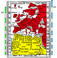
At the head of this article is a Mercator projection truncated at such high latitudes (85N and 85S) that the gross distortion near the poles is clearly apparent. At the same time, the projection is highly accurate near the equator where low scale distortion and conformality guarantee good shape reproduction. Africa is at the centre of the map and it is fairly true to shape (as viewed on a globe). Unfortunately the version of the Mercator map which dominated the schoolroom for almost 200 years was truncated asymmetrically. The example shown below, from a Finnish encyclopedia printed in the 1920s, is truncated at approximately 74N and 55S with the result that Africa is displaced from the centre by an enlarged Europe. (Note the varying bar scales on this map, clearly visible in the source file at its highest resolution). This euro-centric world map was criticised by Arno Peters and he advocated the use of an equal area projection which (unknown to Peters) had been developed by the Edinburgh clergyman James Gall in 1855. An example showing national boundaries is shown below. Unfortunately the property of equal area can only be obtained at the expense of conformality and the Gall-Peters projection shows a greatly distorted African continent and moreover it has the pronounced scale distortion at high latitudes common to all cylindric projections. It is now accepted that all cylindric projections are unsuitable for world maps. In 1989 a resolution (here) by seven North American geographical groups mooted the adoption of various non-cylindric world maps and the example below (showing Ultra prominent mountains) is a Winkel Tripel projection--a projection which has been adopted by the National Geographic Society of America.

World maps on Mercator, Gall--Peters and Winkel Tripel projections

Google maps

Google Maps currently uses a variant of the Mercator projection for its map images. Despite its obvious scale variation at small scales, the projection is well-suited as an interactive world map that can be zoomed seamlessly to large-scale (local) maps, where there is relatively little distortion due to the projection's near-conformality. (Google Satellite Maps, on the other hand, used a plate carrée projection until July 22, 2005.)

The Google Maps tiling system displays most of the world at zoom level 0 as a single 256 pixel-square image, excluding the polar regions. (The projection shown at the #head of this article illustrates such a 1:1 aspect ratio obtained by truncation at 85N and 85S.

The spherical model

Although the surface of Earth is best modelled by an oblate ellipsoid of revolution, for small scale maps the ellipsoid is approximated by a sphere of radius a. Many different ways exist for calculating a. The simplest include (a) the equatorial radius of the ellipsoid, (b) the arithmetic or geometric mean of the semi-axes of the ellipsoid, (c) the radius of the sphere having the same volume as the ellipsoid.^[17] The range of all possible choices is about 35 km, but for small scale (large region) applications the variation may be ignored, and mean values of 6,371 km and 40,030 km may be taken for the radius and circumference respectively. These are the values used for numerical examples in later sections. Only high-accuracy cartography on large scale maps requires an ellipsoidal model.

Cylindrical projections

The Earth can be modelled by a small sphere of radius R, called the globe in this section. The various cylindrical projections specify how the geographic detail is transferred from the globe to a cylinder tangential to it at the equator. The cylinder is then unrolled to give the planar map.^[18][19] The fraction R/a is called the representative fraction (RF) or the principal scale of the projection. For example, a Mercator map printed in a book might have an equatorial width of 13.4 cm corresponding to a globe radius of 2.13 cm and an RF of approximately 1/300M (M is used as an abbreviation for 1,000,000 in writing an RF) whereas Mercator's original 1569 map has a width of 198 cm corresponding to a globe radius of 31.5 cm and an RF of about 1/20M.

A cylindrical map projection is specified by formulæ linking the geographic coordinates of latitude φ and longitude λ to Cartesian coordinates on the map with origin on the equator and x-axis along the equator. By construction, all points on the same meridian lie on the same generator^[20] of the cylinder at a constant value of x, but the distance y along the generator (measured from the equator) is an arbitrary^[21] function of latitude, y(φ). In general this function does not describe the geometrical projection (as of light rays onto a screen) from the centre of the globe to the cylinder, which is only one of an unlimited number of ways to conceptually project a cylindrical map.

Since the cylinder is tangential to the globe at the equator, the scale factor between globe and cylinder is unity on the equator but nowhere else. In particular since the radius of a parallel, or circle of latitude, is a cos φ, the corresponding parallel on the map must have been stretched by a factor of 1/cos φ = sec φ. This scale factor on the parallel is conventionally denoted by k and the corresponding scale factor on the meridian is denoted by h.^[22]

The relations between y(φ) and properties of the projection, such as the transformation of angles and the variation in scale, follow from the geometry of corresponding small elements on the globe and map. The figure below shows a point P at latitude φ and longitude λ on the globe and a nearby point Q at latitude φ+δφ and longitude λ+δλ. The lines PK and MQ are arcs of meridians of length Rδφ where R is the radius of the globe and φ is in radian measure: the lines PM and KQ are arcs of parallel circles of length R(cos φ)δλ with λ in radian measure. The corresponding points on the projection define a rectangle of width δx and height δy.

For small elements the angle PMQ is approximately a right angle and therefore

${\displaystyle \tan \alpha \approx {\frac {R\cos \phi \,\delta \lambda }{R\,\delta \phi }},\qquad \qquad \tan \beta ={\frac {\delta x}{\delta y}},}$

parallel scale factor     ${\displaystyle \quad k(\phi )\;=\;{\frac {P'M'}{PM}}\;=\;{\frac {\delta x}{R\cos \phi \,\delta \lambda }},}$

meridian scale factor   ${\displaystyle \quad h(\phi )\;=\;{\frac {P'K'}{PK}}\;=\;{\frac {\delta y}{R\delta \phi \,}}.}$

Since the meridians are mapped to lines of constant x we must have x=R(λ-λ₀) and δx=Rδλ, (λ in radians). Therefore in the limit of infinitesimally small elements

${\displaystyle \tan \beta ={\frac {R\sec \phi }{y'(\phi )}}\tan \alpha \,,\qquad k\;=\,\sec \phi \,,\qquad h\;=\;{\frac {y'(\phi )}{R}}.}$

Derivation of the Mercator projection

The choice of the function y(φ) for the Mercator projection is determined by the demand that the projection be conformal, a condition which can be defined in two equivalent ways:

• Equality of angles. The condition that a sailing course of constant azimuth α on the globe is mapped into a constant grid bearing β on the map. Setting α=β in the above equations gives y'(φ)=R secφ.
• Isotropy of scale factors. This is the statement that the point scale factor is independent of direction so that small shapes are preserved by the projection. Setting h=k in the above equations again gives y'(φ)=R secφ.

Integrating the equation

${\displaystyle y'(\phi )=R\sec \phi ,}$

with y(0)=0, by using integral tables^[23] or elementary methods,^[24] gives y(φ). Therefore

${\displaystyle {\begin{aligned}x&=R(\lambda -\lambda _{0}),\qquad y=R\ln \left[\tan \left({\frac {\pi }{4}}+{\frac {\phi }{2}}\right)\right].\end{aligned}}}$

In the first equation λ₀ is the longitude of an arbitrary central meridian usually, but not always, that of Greenwich (i.e. zero). The difference (λ-λ₀) is in radians.

The function y(φ) is plotted alongside for the case R=1: it tends to infinity at the poles. The linear y-axis values are not usually shown on printed maps; instead some maps show the non-linear scale of latitude values on the right. More often than not the maps show only a graticule of selected meridians and parallels

Inverse transformations

${\displaystyle \lambda =\lambda _{0}+{\frac {x}{R}},\qquad \phi =2\tan ^{-1}\left[\exp \left({\frac {y}{R}}\right)\right]-{\frac {\pi }{2}}}$

The expression on the right of the second equation defines the gudermannian function, i.e. φ=gd(y/R): the direct equation may therefore be written as y=R.gd^-1(φ). ^[23]

Alternative expressions

There are many alternative expressions for y(φ), all derived by elementary manipulations.^[24]

${\displaystyle {\begin{aligned}y&=&{\frac {R}{2}}\ln \left[{\frac {1+\sin \phi }{1-\sin \phi }}\right]&=&{R}\ln \left[{\frac {1+\sin \phi }{\cos \phi }}\right]&=R\ln \left(\sec \phi +\tan \phi \right)\\[2ex]&=&R\tanh ^{-1}\!\left(\sin \phi \right)&=&R\sinh ^{-1}\!\left(\tan \phi \right)&=R\cosh ^{-1}\!\left(\sec \phi \right)=R\;{\mbox{gd}}^{-1}(\phi ).\end{aligned}}}$

Corresponding inverses are:

${\displaystyle {\begin{aligned}\phi &=\sin ^{-1}\left[\tanh(y/R)\right]=\tan ^{-1}\left[\sinh(y/R)\right]=\sec ^{-1}\left[\cosh(y/R)\right]={\mbox{gd}}(y/R).\end{aligned}}}$

For angles expressed in degrees:

${\displaystyle {\begin{aligned}x={\frac {\pi R(\lambda ^{\circ }-\lambda _{0}^{\circ })}{180}},\qquad \quad y=R\ln \left[\tan \left(45+{\frac {\phi ^{\circ }}{2}}\right)\right].\end{aligned}}}$

The above formulae are written in terms of the globe radius R. It is often convenient to work directly with the map width W=2πR. For example the basic transformation equations become

${\displaystyle {\begin{aligned}x&={\frac {W}{2\pi }}\left(\lambda -\lambda _{0}\right),\qquad y={\frac {W}{2\pi }}\ln \left[\tan \left({\frac {\pi }{4}}+{\frac {\phi }{2}}\right)\right].\end{aligned}}}$

Truncation and aspect ratio

The ordinate y of the Mercator becomes infinite at the poles and the map must be truncated at some latitude less than ninety degrees. This need not be done symmetrically. Mercator's original map is truncated at 80°N and 66°S with the result that European countries were moved towards the centre of the map. The aspect ratio of his map is 198/120=1.65. Even more extreme truncations have been used: a Finnish school atlas was truncated at approximately 76°N and 56°S, an aspect ratio of 1.97.

Much web based mapping uses a zoomable version of the Mercator projection with an aspect ratio of unity. In this case the maximum latitude attained must correspond to y=±W/2, or equivalently y/R=π. Any of the inverse transformation formulae may be used to calculate the corresponding latitudes:

${\displaystyle \phi =\tan ^{-1}\left[\sinh(y/R)\right]=\tan ^{-1}\left[\sinh \pi \right]=\tan ^{-1}\left[11.5487\right]=85.05113^{\circ }.}$

Scale factor

The figure comparing the infinitesimal elements on globe and projection shows that when α=β the triangles PQM and P'Q'M' are similar so that the scale factor in an arbitrary direction is the same as the parallel and meridian scale factors:

${\displaystyle {\frac {\delta s'}{\delta s}}={\frac {P'Q'}{PQ}}={\frac {P'M'}{PM}}=k={\frac {P'K'}{PK}}=h=\sec \phi .}$

This result holds for an arbitrary direction: the definition of isotropy of the point scale factor. The graph shows the variation of the scale factor with latitude. Some numerical values are listed below.

at latitude 30° the scale factor is   k= sec 30°=1.15,

at latitude 45° the scale factor is   k= sec 45°=1.41,

at latitude 60° the scale factor is   k= sec 60°=2,

at latitude 80° the scale factor is   k= sec 80°=5.76,

at latitude 85° the scale factor is   k= sec 85°=11.5

Working from the projected map requires the scale factor in terms of the Mercator ordinate y (unless the map is provided with an explicit latitude scale). Since ruler measurements can furnish the map ordinate y and also the width W of the map then y/R=2πy/W and the scale factor is determined using one of the alternative forms for the forms of the inverse transformation:

${\displaystyle k=\sec \phi =\cosh(y/R)=\cosh(2\pi y/W).}$

The variation with latitude is sometimes indicated by multiple bar scales as shown below and, for example, on a Finnish school atlas. The interpretation of such bar scales is non-trivial. See the discussion on distance formulae below.

Area scale

The area scale factor is the product of the parallel and meridian scales hk=sec²φ. For Greenland, taking 73° as a median latitude, hk= 11.7. For Australia, taking 25° as a median latitude, hk= 1.2. For Great Britain, taking 55° as a median latitude, hk= 3.04.

Distortion

The classic way of showing the distortion inherent in a projection is to use Tissot's indicatrix. Nicolas Tissot noted that for cylindrical projections the scale factors at a point, specified by the numbers h and k, define an ellipse at that point of the projection. The axes of the ellipse are aligned to the meridians and parallels.^[22][25][26] For the Mercator projection, h=k, so the ellipses degenerate into circles with radius proportional to the value of the scale factor for that latitude. These circles are then placed on the projected map with an arbitrary overall scale (because of the extreme variation in scale) but correct relative sizes.

Accuracy

One measure of a map's accuracy is a comparison of the length of corresponding line elements on the map and globe. Therefore, by construction, the Mercator projection is perfectly accurate, k=1, along the equator and nowhere else. At a latitude of ±25° the value of sec φ is about 1.1 and therefore the projection may be deemed accurate to within 10% in a strip of width 50° centred on the equator. Narrower strips are better: sec 8°=1.01, so a strip of width 16° (centred on the equator) is accurate to within 1% or 1 part in 100. Similarly sec 2.56°=1.001, so a strip of width 5.12° (centred on the equator) is accurate to within 0.1% or 1 part in 1,000. Therefore the Mercator projection is adequate for mapping countries close to the equator.

Secant projection

In a secant (in the sense of cutting) Mercator projection the globe is projected to a cylinder which cuts the sphere at two parallels with latitudes ±φ₁. The scale is now true at these latitudes whereas parallels between these latitudes are contracted by the projection and their scale factor must be less than one. The result is that deviation of the scale from unity is reduced over a wider range of latitudes.

An example of such a projection is

${\displaystyle x=0.99R\lambda \qquad y=0.99R\ln \tan \!\left({\frac {\pi }{4}}+{\frac {\phi }{2}}\right)\qquad k\;=0.99\sec \phi .}$

The scale on the equator is 0.99; the scale is k=1 at a latitude of approximately ±8° (the value of φ₁); the scale is k=1.01 at a latitude of approximately ±11.4°. Therefore the projection has an accuracy of 1%, over a wider strip of 22° compared with the 16° of the normal (tangent) projection.This is a standard technique of extending the region over which a map projection has a given accuracy.

Generalisation to the ellipsoid

When the Earth is modelled by an ellipsoid (of revolution) the Mercator projection must be modified if it is to remain conformal. The transformation equations and scale factor for the non-secant version are^[27]

${\displaystyle {\begin{aligned}x&=R\left(\lambda -\lambda _{0}\right),\\y&=R\ln \left[\tan \left({\frac {\pi }{4}}+{\frac {\phi }{2}}\right)\left({\frac {1-e\sin \phi }{1+e\sin \phi }}\right)^{e/2}\right],\\k&=\sec \phi {\sqrt {1-e^{2}\sin ^{2}\phi }}.\end{aligned}}}$

The scale factor is unity on the equator, as it must be since the cylinder is tangential to the ellipsoid at the equator. The ellipsoidal correction of the scale factor increases with latitude but it is never greater than e², a correction of less than 1%. (The value of e² is about 0.006 for all reference ellipsoids.) This is much smaller than the scale inaccuracy, except very close to the equator. Accurate Mercator projections of regions near the equator will necessitate the ellipsoidal corrections.

Formulæ for distance

Converting ruler distance on the Mercator map into true (great circle) distance on the sphere is straightforward along the equator but nowhere else. One problem is the variation of scale with latitude, and another is that straight lines on the map (rhumb lines), other than the meridians or the equator, do not correspond to great circles.

The distinction between rhumb (sailing) distance and great circle (true) distance was clearly understood by Mercator. (See Legend 12 on the 1569 map.) He stressed that the rhumb line distance is an acceptable approximation for true great circle distance for courses of short or moderate distance, particularly at lower latitudes. He even quantifies his statement: "When the great circle distances which are to be measured in the vicinity of the equator do not exceed 20 degrees of a great circle, or 15 degrees near Spain and France, or 8 and even 10 degrees in northern parts it is convenient to use rhumb line distances".

For a ruler measurement of a short line, with mid-point at latitude φ, where the scale factor is k=secφ = 1/cos φ:

True distance = rhumb distance ≅ ruler distance * cos φ / RF.   (short lines)

With radius and great circle circumference equal to 6,371 km and 40,030 km respectively an RF of 1/300M, for which R=2.12 cm and W=13.34 cm, implies that a ruler measurement of 3 mm. in any direction from a point on the equator corresponds to approximately 900 km. The corresponding distances for latitudes 20°, 40°, 60° and 80° are 846 km, 689 km, 450 km and 156 km respectively.

Longer distances require various approaches.

On the equator

Scale is unity on the equator (for a non-secant projection). Therefore interpreting ruler measurements on the equator is simple:

True distance = ruler distance / RF     (equator))

For the above model, with RF=1/300M, 1 cm corresponds to 3,000 km.

On other parallels

On any other parallel the scale factor is secφ so that

Parallel distance = ruler distance * cos φ / RF     (parallel))

For the above model 1 cm corresponds to 1,500 km at a latitude of 60°.

This is not the shortest distance between the chosen endpoints on the parallel because a parallel is not a great circle. The difference is small for short distances but increases as λ, the longitudinal separation, increases. For two points, A and B, separated by 10° of longitude on the parallel at 60° the distance along the parallel is approximately 0.5 km greater than the great circle distance. (The distance AB along the parallel is (a cosφ) λ. The length of the chord AB is 2(a cosφ)sin(λ/2). This chord subtends an angle at the centre equal to 2arcsin( cosφ sin(λ/2)) and the great circle distance between A and B is 2a arcsin( cosφ sin(λ/2)).) In the extreme case where the longitudinal separation is 180°, the distance along the parallel is one half of the circumference of that parallel, i.e. 10,007.5 km. On the other hand the geodesic between these points is a great circle arc through the pole subtending an angle of 60° at the center: the length of this arc is one sixth of the great circle circumference, about 6,672 km. The difference is 3,338 km so the ruler distance measured from the map is quite misleading even after correcting for the latitude variation of the scale factor.

On a meridian

A meridian of the map is a great circle on the globe but the continuous scale variation means ruler measurement alone cannot yield the true distance between distant points on the meridian. However, if the map is marked with an accurate and finely spaced latitude scale from which the latitude may be read directly—as is the case for the Mercator 1569 world map (sheets 3, 9, 15) and all subsequent nautical charts—the meridian distance between two latitudes φ₁ and φ₂ is simply

${\displaystyle m_{12}=a|\phi _{1}-\phi _{2}|.}$

If the latitudes of the end points cannot be determined with confidence then they can be found instead by calculation on the ruler distance. Calling the ruler distances of the end points on the map meridian as measured from the equator y₁ and y₂, the true distance between these points on the sphere is given by using any one of the inverse Mercator formulæ:

${\displaystyle m_{12}=a\left|\tan ^{-1}\left[\sinh({y_{1}}/{R})\right]-\tan ^{-1}\left[\sinh({y_{2}}/{R})\right]\right|,}$

where R may be calculated from the width W of the map by R=W/2π. For example, on a map with R=1 the values of y=0, 1, 2, 3 correspond to latitudes of φ=0°, 50°, 75°, 84° and therefore the successive intervals of 1 cm on the map correspond to latitude intervals on the globe of 50°, 25°, 9° and distances of 5,560 km, 2,780 km, and 1,000 km on the Earth.

On a rhumb

A straight line on the Mercator map at angle α to the meridians is a rhumb line. When α=π/2 or 3π/2 the rhumb corresponds to one of the parallels; only one, the equator, is a great circle. When α=0 or π it corresponds to to a meridian great circle (if continued around the Earth). For all other values it is a spiral from pole to pole on the globe intersecting the meridians at the same angle: it is not a great circle.^[24] This section discusses only the last of these cases.

If α is neither 0 nor π then figure of the infinitesimal elements shows that the length of an infinitesimal rhumb line on the sphere between latitudes φ and φ+δφ is a secα δφ. Since α is constant on the rhumb this expression can be integrated to give, for finite rhumb lines on the Earth:

${\displaystyle r_{12}=a\sec \alpha \,|\phi _{1}-\phi _{2}|=a\,\sec \alpha \;\Delta \phi .}$

Once again, if Δφ may be read directly from an accurate latitude scale on the map, then the rhumb distance between map points with latitudes φ₁ and φ₂ is given by the above. If there is no such scale then the ruler distances between the end points and the equator, y₁ and y₂, give the result via an inverse formula:

${\displaystyle r_{12}=a\sec \alpha \left|\tan ^{-1}\sinh(y_{1}/R)-\tan ^{-1}\sinh(y_{2}/R)\right|.}$

These formulæ give rhumb distances on the sphere which may differ greatly from true distances whose determination requires more sophisticated calculations.^[28]

• Maling, Derek Hylton (1992), Coordinate Systems and Map Projections (second ed.), Pergamon Press, ISBN 0-08-037033-3 {{citation}}: Check |isbn= value: checksum (help).
• Olver, F. W.J.; Lozier, D.W.; Boisvert, R.F.; Clark, C.W., eds. (2010,), NIST Handbook of Mathematical Functions, Cambridge University Press {{citation}}: Check date values in: |year= (help)CS1 maint: extra punctuation (link)
• Osborne, Peter (2008), The Mercator Projections. {{citation}}: External link in |publisher= (help); Missing or empty |title= (help)
• Rapp, Richard H (1991), Geometric Geodesy, Part I, [http://hdl.handle.net/1811/24333 {{citation}}: External link in |publisher= (help)
• Snyder, John P (1993), Flattening the Earth: Two Thousand Years of Map Projections, University of Chicago Press, ISBN 0-226-76747-7
• Snyder, John P. (1987), Map Projections – A Working Manual. U.S. Geological Survey Professional Paper 1395, United States Government Printing Office, Washington, D.C.This paper can be downloaded from USGS pages. It gives full details of most projections, together with interesting introductory sections, but it does not derive any of the projections from first principles.

• Cartography
• Cassini projection
• Dymaxion map
• Equirectangular projection
• Gall-Peters projection with resolution regarding the use of rectangular world maps
• Gnomonic projection
• Lambert conformal conic projection (used extensively in aviation)
• Map projection
• Mollweide projection
• Nautical chart
• Robinson projection
• Reversed map
• Transverse Mercator projection
• Winkel Tripel projection

• Snyder, John P. (1987). Map Projections - A Working Manual. U.S. Geological Survey Professional Paper 1395. United States Government Printing Office, Washington, D.C. This paper can be downloaded from USGS pages.
• Monmonier, Mark (2004). Rhumb Lines and Map Wars. Chicago: The University of Chicago Press.
• Needham, Joseph (1986). Science and Civilization in China: Volume 3; Mathematics and the Sciences of the Heavens and the Earth. Taipei: Caves Books Ltd.
• Needham, Joseph (1986). Science and Civilization in China: Volume 4, Physics and Physical Technology, Part 3, Civil Engineering and Nautics. Taipei: Caves Books Ltd.
• Google Maps Coordinates
• Gerard Mercator, 1538. World Map. In Fite & Freeman, A Book of Old Maps. 1926. Cambridge: Harvard University Press.

• Ad maiorem Gerardi Mercatoris gloriam - contains high resolution images of the 1569 world map by Mercator.
• Table of examples and properties of all common projections, from radicalcartography.net.
• An interactive Java Applet to study the metric deformations of the Mercator Projection.

• Brigitte English, Erhard Etzlaub's Projection and Methods of Mapping, in: Imago Mundi, 48 (1996), pp. 103–123.

• Mercator in the German National Library catalogue

[1]

• Fritz Schnelbögl, „Leben und Werk des Nürnberger Kartographen Erhard Etzlaub“ in Mitteilungen des Vereins für Geschichte der Stadt Nürnberg Bd. 57. 1970, S. 216-231, Facsimile, German.
• F.W. Krücken, Düsseldorf 2004, On Etzlaub's and Mercator's maps, German
• Original woodcut of the "Romweg map"
• Facsimile of the 1500 "Romweg" map, not coloured, but high resolution
• Cut of the 1500 "Romweg" map, coloured
• Cut of the 1501 coloured edition
• 1492, Surroundings of Nuremberg, zoomable map (Österreichische Nationalbibliothek, Vienna, Austria)